You Only Look Twice — Multi-Scale Object Detection in Satellite Imagery With Convolutional Neural Networks (Part I)

Detection of small objects over large swaths is one of the primary drivers of interest in satellite imagery analytics. Previous posts (4, 5) detailed efforts to localize boats in DigitalGlobe images using sliding windows and HOG feature descriptors. These efforts proved successful in both open water and harbor regions, though such techniques struggle in regions of highly non-uniform background. To address the shortcomings of classical object detection techniques we implement an object detection pipeline based upon the You Only Look Once framework. This pipeline (which we dub You Only Look Twice) greatly improves background discrimination over the HOG-based approach, and proves able to rapidly detect objects of vastly different scales and over multiple sensors.

1. Satellite Imagery Object Detection Overview

The ImageNet competition has helped spur rapid advancements in the field of computer vision object detection, yet there are a few key differences between the ImageNet data corpus and satellite imagery. Four issues create difficulties: in satellite imagery objects are often very small (~20 pixels in size), they are rotated about the unit circle, input images are enormous (often hundreds of megapixels), and there’s a relative dearth of training data (though efforts such as SpaceNet are attempting to ameliorate this issue). On the positive side, the physical and pixel scale of objects are usually known in advance, and there’s a low variation in observation angle. One final issue of note is deception; observations taken from hundreds of kilometers away can sometimes be easily fooled. In fact, the front page of The New York Times on October 13, 2016 featured a story about Russian weapon mock-ups (Figure 1).

2. HOG Boat Detection Challenges

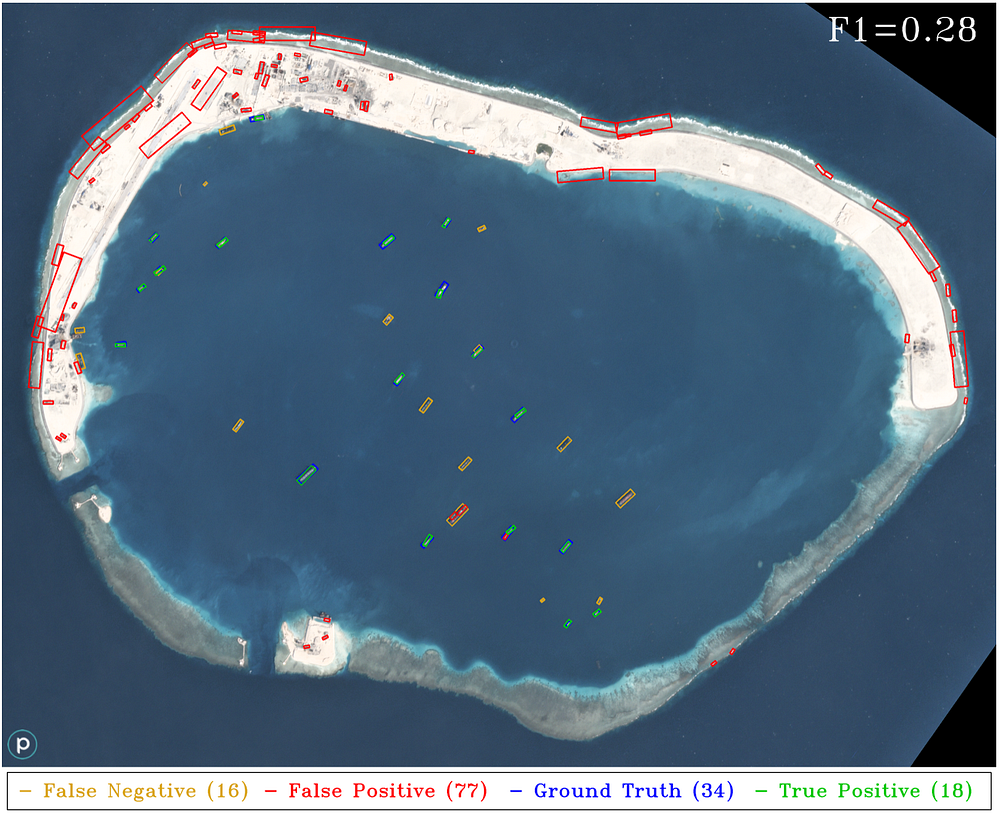
The HOG + Sliding Window object detection approach discussed in previous posts (4, 5) demonstrated impressive results in both open water and harbor (F1 ~ 0.9). Recall from Section 2 of 5 that we evaluate true and false positives and negatives by defining a true positive as having a Jaccard index (also known as intersection over union) of greater than 0.25. Also recall that the F1 score is the harmonic mean of precision and recall and varies from 0 (all predictions are wrong) to 1 (perfect prediction).

To explore the limits of the HOG + Sliding Window pipeline, we apply it to a scene with a less uniform background and from a different sensor. Recall that our classifier was trained on DigitalGlobe data with 0.5 meter ground sample distance (GSD), though our test image below is a Planet image at 3m GSD.

3. Object Detection With Deep Learning

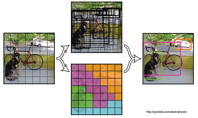
We adapt the You Only Look Once (YOLO) framework to perform object detection on satellite imagery. This framework uses a single convolutional neural network (CNN) to predict classes and bounding boxes. The network sees the entire image at train and test time, which greatly improves background differentiation since the network encodes contextual information for each object. It utilizes a GoogLeNet inspired architecture, and runs at real-time speed for small input test images. The high speed of this approach combined with its ability to capture background information makes for a compelling case for use with satellite imagery.

The attentive reader may wonder why we don’t simply adapt the HOG + Sliding Window approach detailed in previous posts to instead use a deep learning classifier rather than HOG features. A CNN classifier combined with a sliding window can yield impressive results, yet quickly becomes computationally intractable. Evaluating a GoogLeNet-based classifier is roughly 50 times slower on our hardware than a HOG-based classifier; evaluation of Figure 2 changes from ~2 minutes for the HOG-based classifier to ~100 minutes. Evaluation of a single DigitalGlobe image of ~60 square kilometers could therefore take multiple days on a single GPU without any preprocessing (and pre-filtering may not be effective in complex scenes). Another drawback to sliding window cutouts is that they only see a tiny fraction of the image, thereby discarding useful background information. The YOLO framework addresses the background differentiation issues, and scales far better to large datasets than a CNN + Sliding Window approach.

The framework does have a few limitations, however, encapsulated by three quotes from the paper:

1. “Our model struggles with small objects that appear in groups, such as flocks of birds”
2. “It struggles to generalize objects in new or unusual aspect ratios or configurations”
3. “Our model uses relatively coarse features for predicting bounding boxes since our architecture has multiple downsampling layers from the original image”

To address these issues we implement the following modifications, which we name YOLT: You Only Look Twice (the reason for the name shall become apparent later):

“Our model struggles with small objects that appear in groups, such as flocks of birds”

• Upsample via a sliding window to look for small, densely packed objects
• Run an ensemble of detectors at multiple scales

“It struggles to generalize objects in new or unusual aspect ratios or configurations”

• Augment training data with re-scalings and rotations

“Our model uses relatively coarse features for predicting bounding boxes since our architecture has multiple downsampling layers from the original image”

• Define a new network architecture such that the final convolutional layer has a denser final grid

The output of the YOLT framework is post-processed to combine the ensemble of results for the various image chips on our very large test images. These modifications reduce speed from 44 frames per second to 18 frames per second. Our maximum image input size is ~500 pixels for NVIDIA GTX Titan X GPU; the high number of parameters for the dense grid we implement saturates the 12GB of memory available on our hardware for images greater than this size. It should be noted that the maximum image size could be increased by a factor of 2–4 if searching for closely packed objects is not required.

4. YOLT Training Data

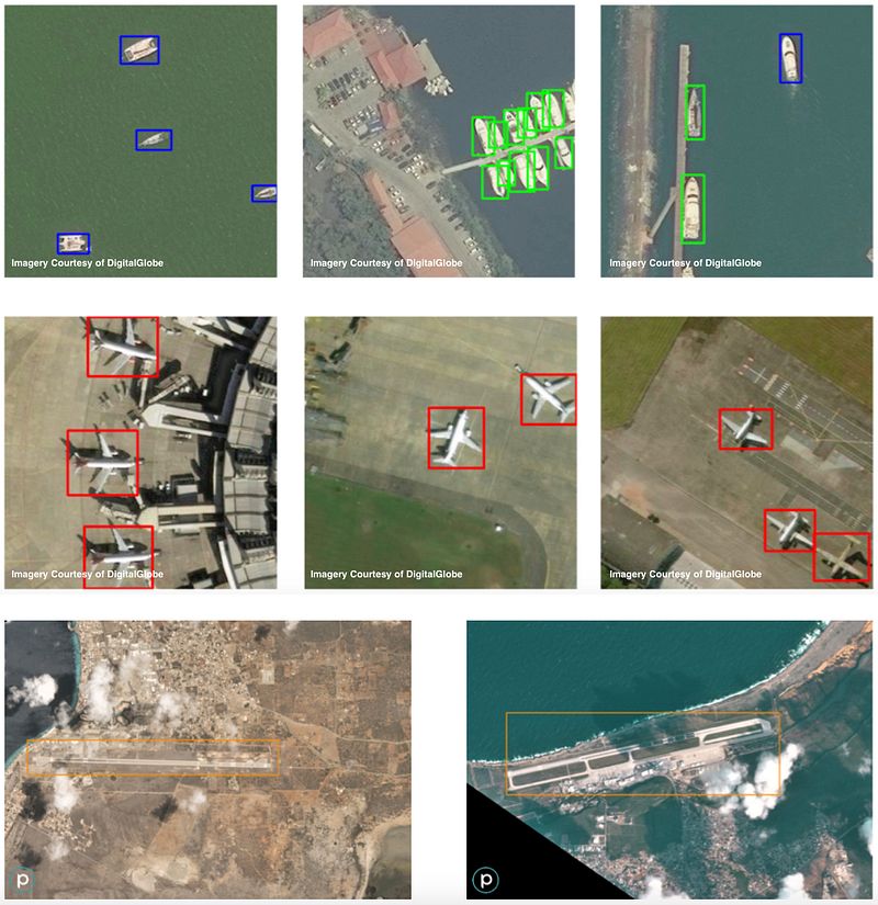
Training data is collected from small chips of large images from both DigitalGlobe and Planet. Labels are comprised of a bounding box and category identifier for each object.

We initially focus on four categories:

• Boats in open water
• Boats in harbor
• Airplanes
• Airports

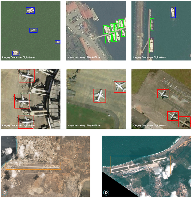
We label 157 images with boats, each with an average of 3–6 boats in the image. 64 image chips with airplanes are labeled, averaging 2–4 airplanes per chip. 37 airport chips are collected, each with a single airport per chip. We also rotate and randomly scale the images in HSV (hue-saturation-value) to increase the robustness of the classifier to varying sensors, atmospheric conditions, and lighting conditions.

With this input corpus training takes 2–3 days on a single NVIDIA Titan X GPU. Our initial YOLT classifier is trained only for boats and airplanes; we will treat airports in Part II of this post. For YOLT implementation we run a sliding window across our large test images at two different scales: a 120 meter window optimized to find small boats and aircraft, and a 225 meter window which is a more appropriate size for larger vessels and commercial airliners.

This implementation is designed to maximize accuracy, rather than speed. We could greatly increase speed by running only at a single sliding window size, or by increasing the size of our sliding windows by downsampling the image. Since we are looking for very small objects, however, this would adversely affect our ability to differentiate small objects of interest (such as 15m boats) from background objects (such as a 15m building). Also recall that raw DigitalGlobe images are roughly 250 megapixels, and inputting a raw image of this size into any deep learning framework far exceeds current hardware capabilities. Therefore either drastic downsampling or image chipping is necessary, and we adopt the latter.

5. YOLT Object Detection Results

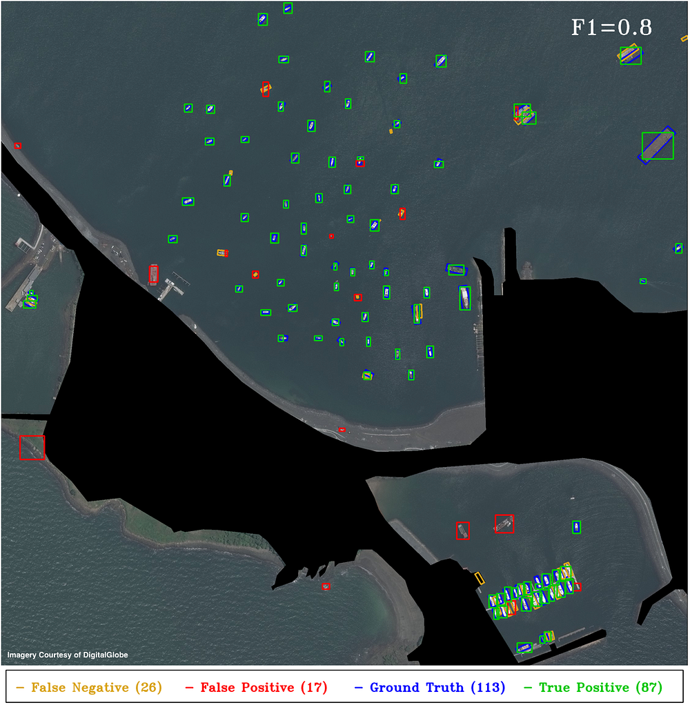
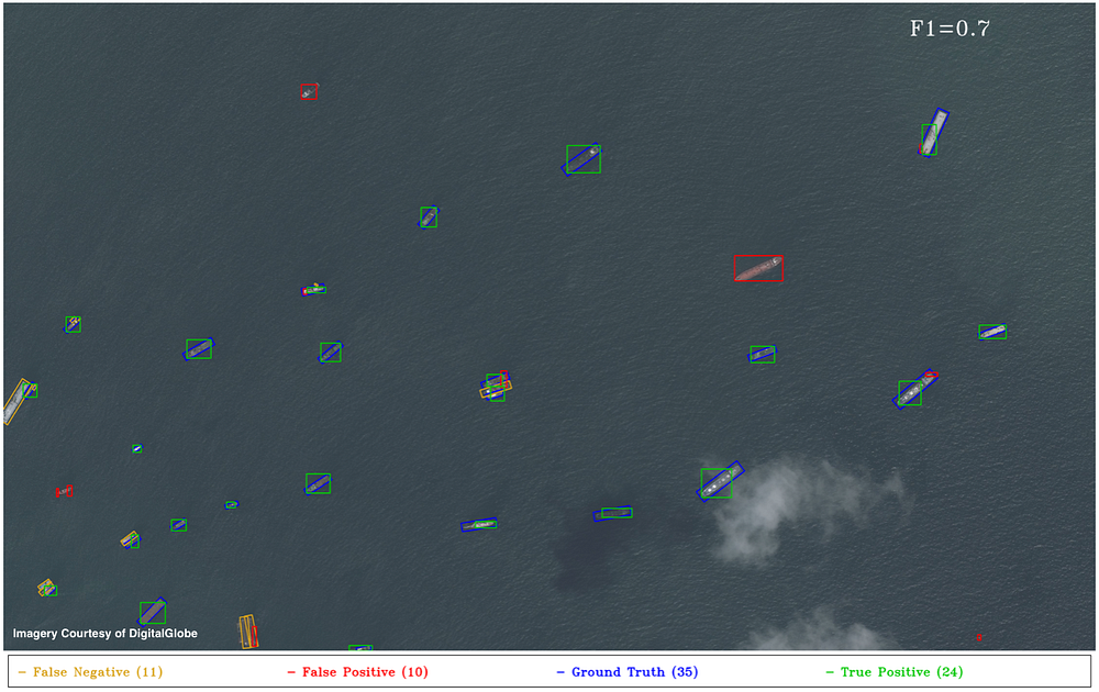
We evaluate test images using the same criteria as Section 2 of 5, also detailed in Section 2 above. For maritime region evaluation we use the same areas of interest as in (4, 5). Running on a single NVIDIA Titan X GPU, the YOLT detection pipeline takes between 4–15 seconds for the images below, compared to the 15–60 seconds for the HOG + Sliding Window approach running on a single laptop CPU. Figures 6–10 below are as close to an apples-to-apples comparison between HOG + Sliding Window and YOLT pipeline as possible, though recall that the HOG + Sliding window is trained to classify the existence and heading of boats, whereas YOLT is trained to produce boat and airplane localizations (not heading angles). All plots use a Jaccard index detection threshold of 0.25 to mimic the results of 5.

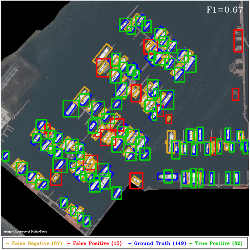
The YOLT pipeline reforms well in open water, though without further post-processing the YOLT pipeline is suboptimal for extremely dense regions, as Figure 9 demonstrates. The four areas of interest discussed above all possessed relatively uniform background, an arena where the HOG + Sliding Window approach performs well. As we showed in Figure 2, however, in areas of highly non-uniform background the HOG + Sliding Window approach struggles to differentiate boats from linear background features; convolutional neural networks offer promise in such scenes.

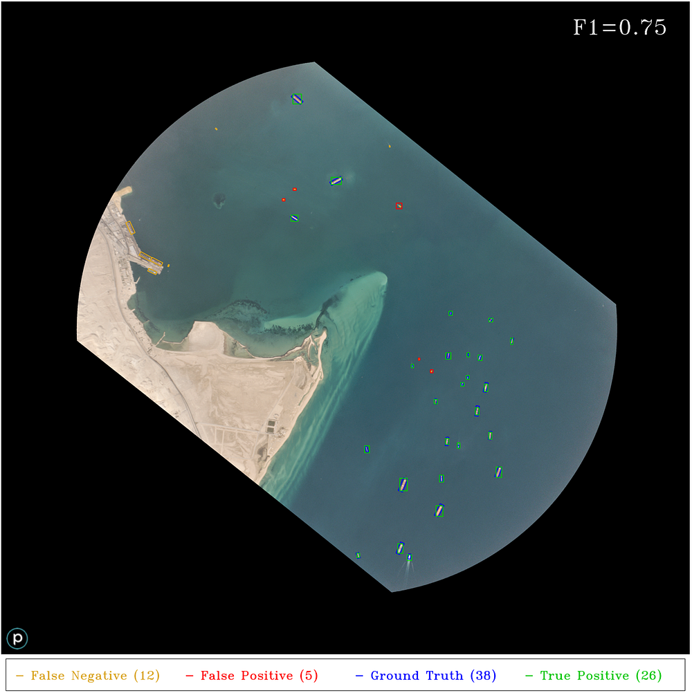
To test the robustness of the YOLT pipeline we analyze another Planet image with a multitude of boats (see Figure 11 below).

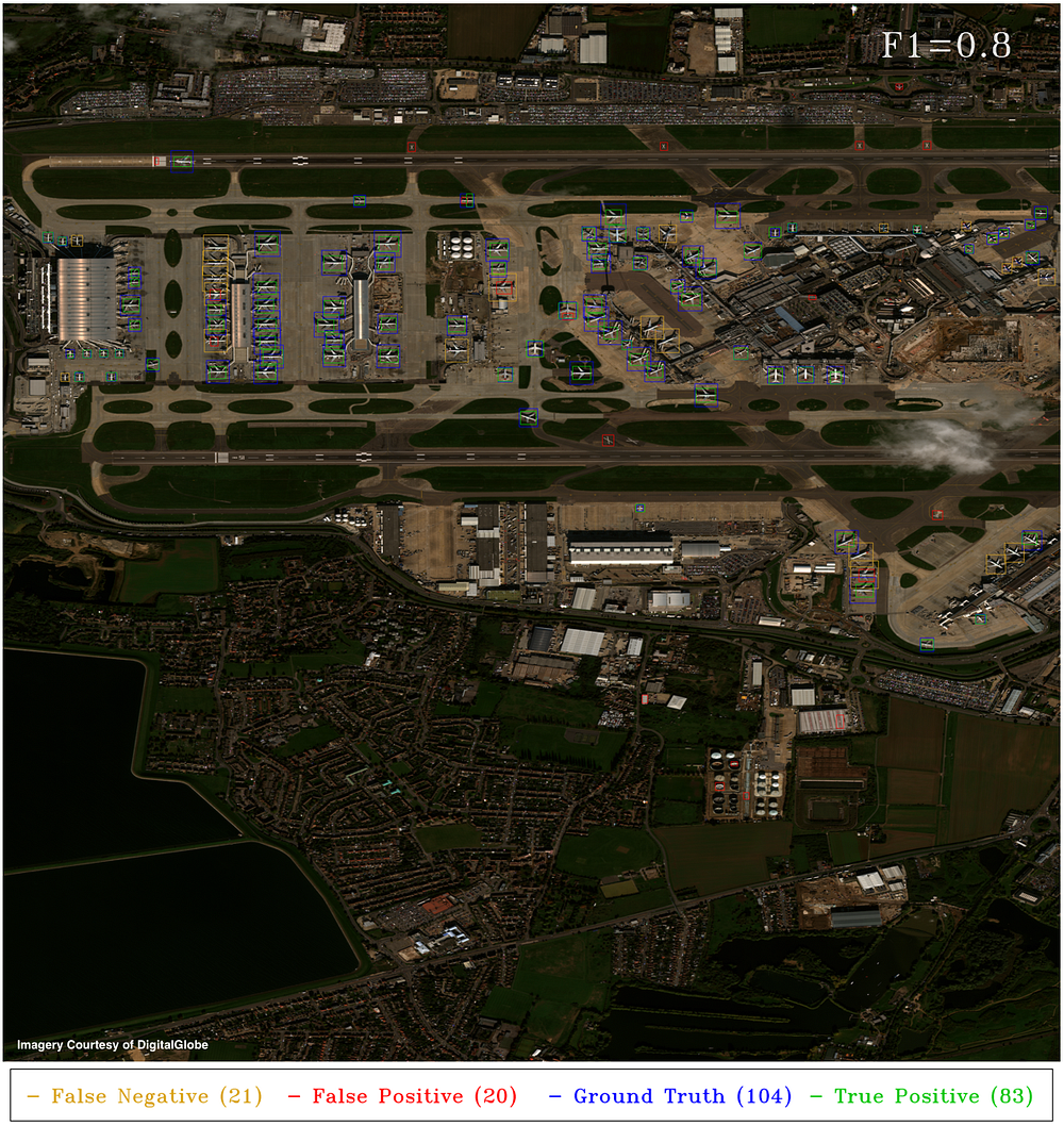
A final test is to see how well the classifier performs on airplanes, as we show below.

6. Conclusion

In this post we demonstrated one of the limitations of classical machine learning techniques as applied to satellite imagery object detection: namely, poor performance in regions of highly non-uniform background. To address these limitations we implemented a fully convolutional neural network classifier (YOLT) to rapidly localize boats and airplanes in satellite imagery. The non-rotated bounding box output of this classifier is suboptimal in very crowded regions, but in sparse scenes the classifier proves far better than the HOG + Sliding Window approach at suppressing background detections and yields an F1 score of 0.7–0.85 on a variety of validation images. We also demonstrated the ability to train on one sensor (DigitalGlobe), and apply our model to a different sensor (Planet). While the F1 scores may not be at the level many readers are accustomed to from ImageNet competitions, we remind the reader that object detection in satellite imagery is a relatively nascent field and has unique challenges, as outlined in Section 1. We have also striven to show both the success and failure modes of our approach. The F1 scores could possibly be improved with a far larger training dataset and further post-processing of detections. Our detection pipeline accuracy might also improve with a greater number of image chips, though this would also reduce the current processing speed of 20–50 square kilometers per minute for objects of size 10m — 100m.

In Part II of this post, we will explore the challenges of simultaneously detecting objects at vastly different scales, such as boats, airplanes, and airstrips.

You Only Look Twice (Part II) — Vehicle and Infrastructure Detection in Satellite Imagery

Rapid detection of objects of vastly different scales over large areas is of great interest in the arena of satellite imagery analytics. In the previous post (6) we implemented a fully convolutional neural network classifier (You Only Look Twice: YOLT) to rapidly localize boats and airplanes in satellite imagery. In this post we detail efforts to extend the YOLT classifier to multiple scales, both at the vehicle level and at infrastructure scales.

1. Combined classifier

Recall that our YOLT training data consists of bounding box delineations of airplanes, boats, and airports.

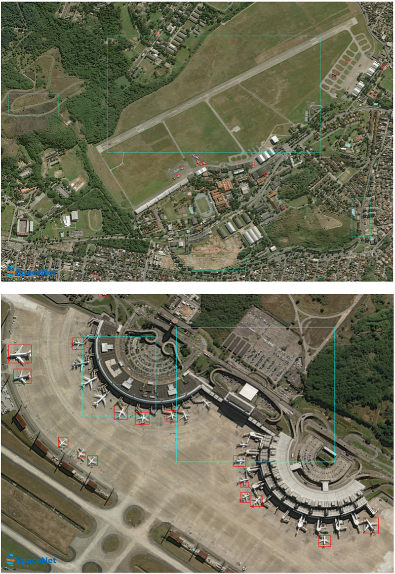
Our previous post (6) demonstrated the ability to localize boats and airplanes via training a 3-class YOLT model. Expanding the model to four classes and including airports is relatively unsuccessful, however, as we show below.

2. Scale Confusion Mitigation

There are multiple ways one could address the false positive issue noted in Figure 2. Recall from 6 that for this exploratory work our training set consists of only a few dozen airports and a couple hundred airplanes, far smaller than usual for deep learning models. Increasing this training set size could greatly improve our model, particularly if the background is highly varied. Another option would be to use post-processing to remove any detections at the incorrect scale (e.g.: an airport with a size of 50 meters). Another option is to simply build dual classifiers, one for each relevant scale. We explore this final option below.

3. Infrastructure Classifier

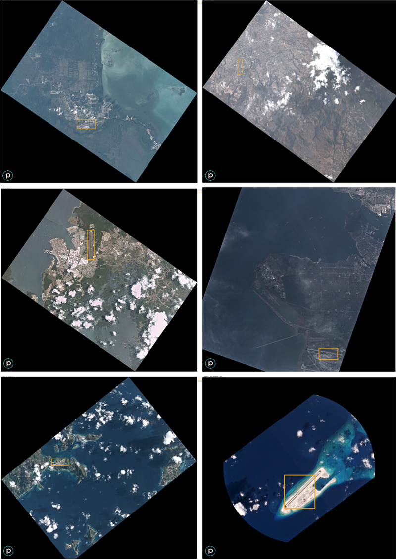
We train a classifier to recognize airports and airstrips using the training data described in 6 of 37 Planet images at ~3m ground sample distance (GSD). These images are augmented by rotations and rescaling in the hue-saturation-value (HSV) space.

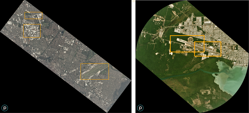
Over the entire corpus of airport test images, we achieve an F1 score of 0.87, and each image takes between 4–10 seconds to analyze depending on size.

4. Dual Classifiers — Infrastructure + Vehicle

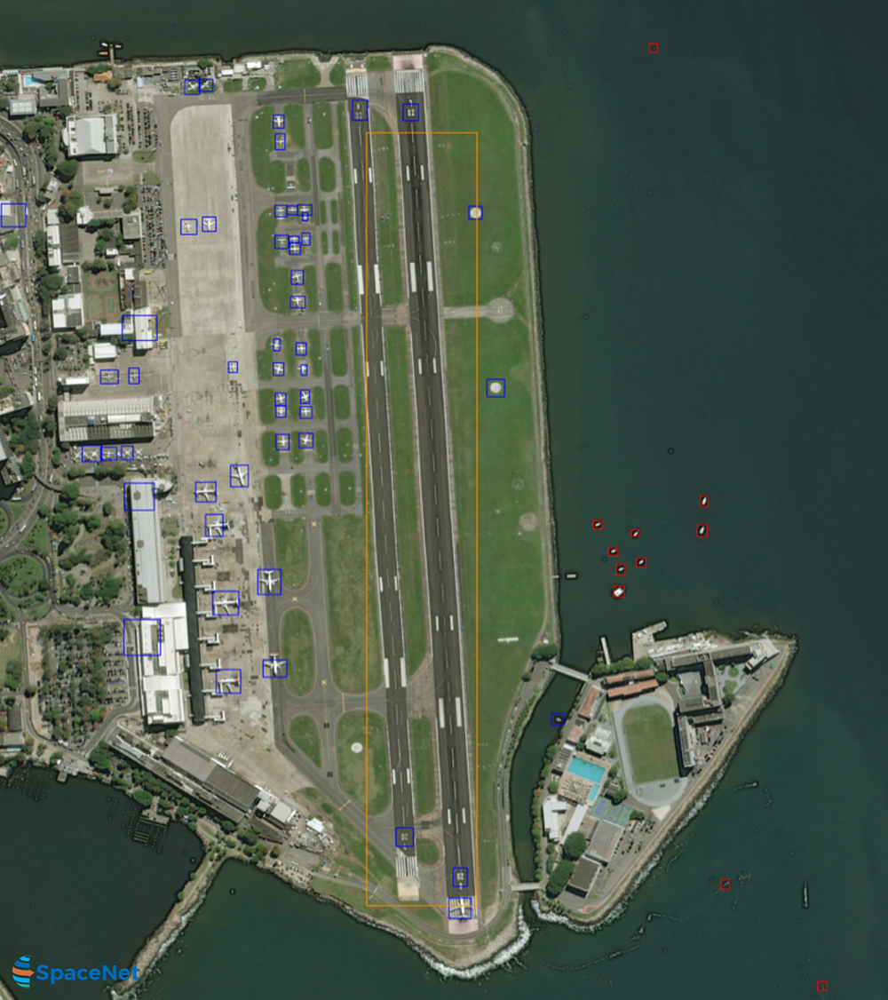
We are now in a position to combine the vehicle-scale classifier trained in 6with the infrastructure classifier of Section 3 above. For large validation images, we run the classifier at three different scales: 120m, 200m, and 2500m. The first scale is designed for small boats, while the second scale captures commercial ships and aircraft, and the largest scale is optimized for large infrastructure such as airports. We break the validation image into appropriately sized bins and run each image chip on the appropriate classifier. The myriad results from the many image chips and multiple classifiers are combined into one final image.

Overlapping detections are merged via non-maximal suppression, and all detections above a certain threshold are plotted. The relative abundances of false positives and false negatives is a function of the probability threshold. A higher threshold means that only highly probable detections are plotted, yielding fewer detections and therefore fewer false positives and more false negatives. A lower threshold yields more detections and therefore more false positives and fewer false negatives. We find a detection probability threshold of between 0.3 and 0.4 yields the highest F1 score for our validation images. Figure 5 below shows all detections above a threshold of 0.3.