Applying Neural Network and Local Laplace Filter Methods to Very High Resolution Satellite Imagery to Detect Damage in Urban Areas
by Dariia Gordiiuk
Since the beginning of the human species, we have been at the whim of Mother Nature. Her awesome power can destroy vast areas and cause chaos for the inhabitants. The use of satellite data to monitor the Earths surface is becoming more and more essential. Of particular importance are the disasters and hurricane monitoring systems that can help people to identify damage in remote areas, measure the consequences of the events, and estimate the overall damage to a given area. From a computing perspective, such an important task needs to be implemented to assist in various situations.
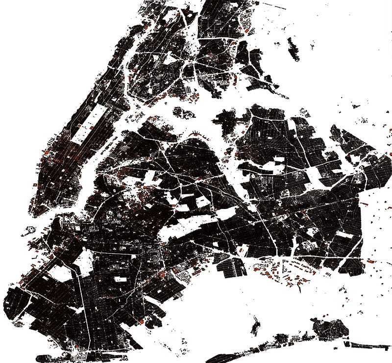
To analyze and estimate the effects of a disaster, we use high-resolution, satellite imagery from an area of interest. This can be obtained from Google Earth. We can also get free OSM vector data that has a detailed ground truth mask of houses. This is the latest vector zip from New York (Figure 1).
Clik here to view.
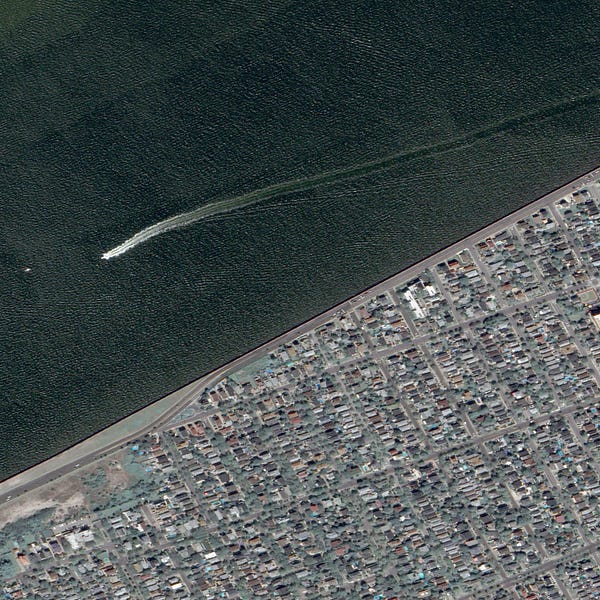
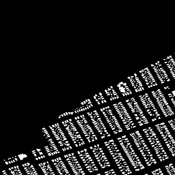
Next, we rasterize (convert from vector to raster) the image using a tool from gdal, called gdal_rasterize. As a result we have acquired a training and testing dataset from Long Island (Figure 2).
Clik here to view.
Clik here to view.
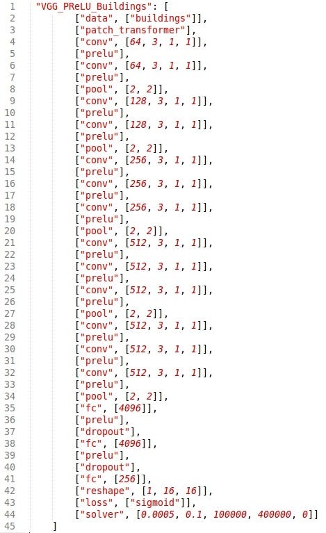
We apply a deep learning framework Caffe for training purposes and the learning model of Convolutional Neural Networks (CNN):
Clik here to view.
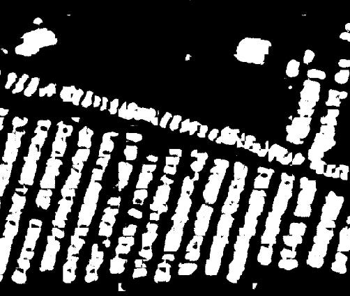
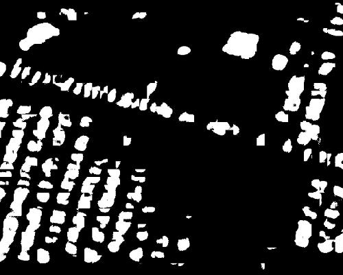
The derived neural net enables us to identify the predicted houses from the target area after the event (Figure 4). We can also use data from another similar area which hasn’t been damaged for CNN learning (if we can’t access the data for the desired territory).
Clik here to view.
Clik here to view.
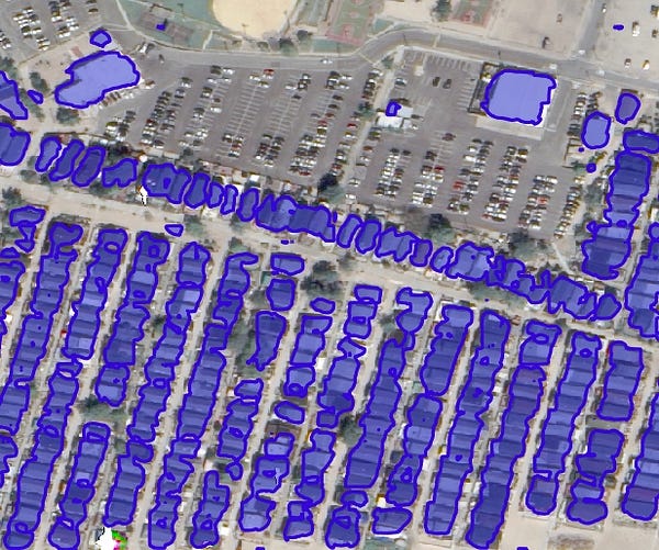
We work with predicates of buildings using vectorization (extracting a contour and then converting lines to polygons) (Figure 5).
Clik here to view.
Clik here to view.
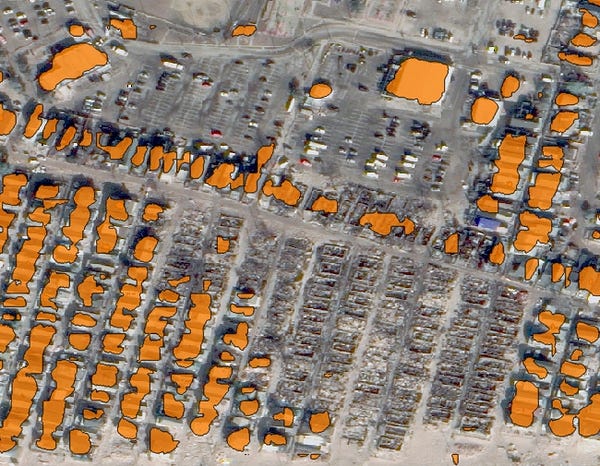
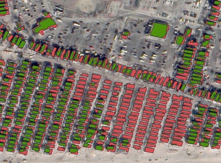
Also, we need to compute the intersection of the obtained predicate vector and the original OSM vector (Figure 6). This task can be accomplished by creating a new filter, dividing the square of the predicate buildings by the original OSM vector. Then, we filter the predictive houses by applying a threshold of 10%. This means that if the area of houses in green (Figure 6) is 10% less than the area in red, the real buildings have been destroyed.
Clik here to view.
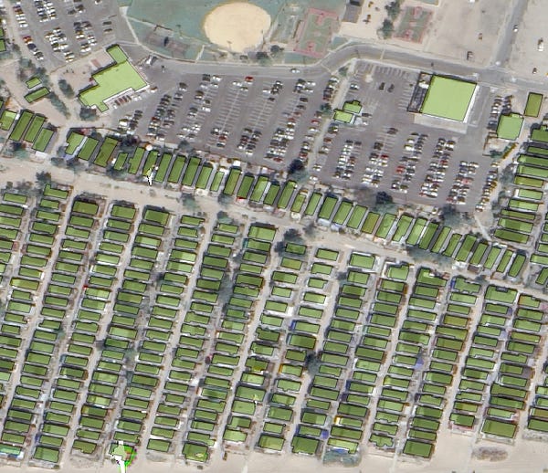
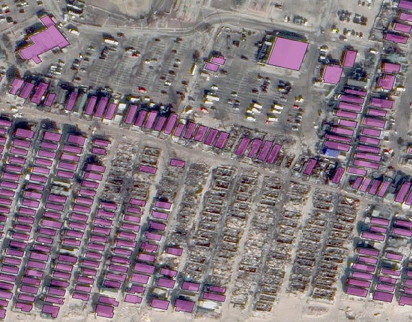
Using the 10%-area threshold we can remove the houses that have been destroyed and get a new map that displays existing buildings (Figure 7). By computing the difference between the pre- and post- disaster masks, we obtain a map of the destroyed buildings (Figure 8).
Clik here to view.
Clik here to view.
Clik here to view.
We have to remember that the roofs of the houses are represented as flat structures in 2D-images. This is an important feature that can also be used to filter input images. A local Laplace filter is a great tool for classifying flat and rough surfaces (Figure 9). The first image has to be a 4-channel image with the fourth Alpha-channel that describes no-data-value pixels in the input image. The second image (img1) is the same, a 3-channel RGB image.
Clik here to view.
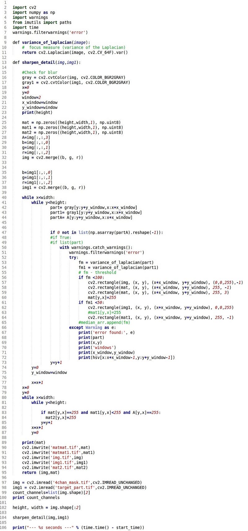
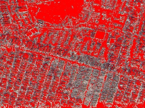
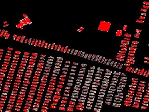
Applying this tool lets you get the map of the flat surface. Let’s look at the new mask of the buildings which have flat and rough textures (Figure 10)after combining this filter and extracting the vector map.
Clik here to view.
Clik here to view.
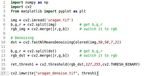
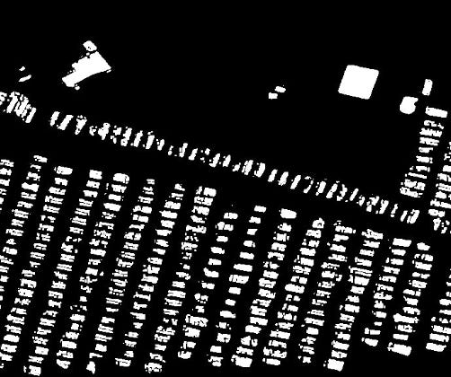
A robust library of the OpenCV computer vision has a denoising filter that helps remove noise from the flat buildings masks (Figure 11, 12).
Clik here to view.
Clik here to view.
Clik here to view.
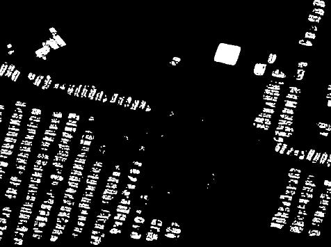
Next, we apply filters to extract the contours and convert the lines into the polygons. This enables us to get new building recognition results (Figure 13).
Clik here to view.
Clik here to view.
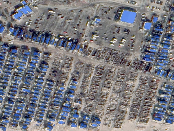
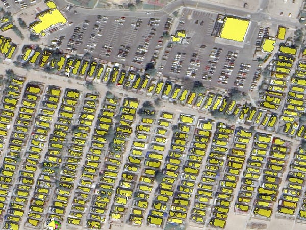
We compute the area of an intersection vector mask obtained from the filter and a ground truth OSM mask and use a 14% threshold to reduce false positives (Figure 14).
Clik here to view.
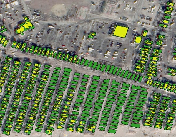
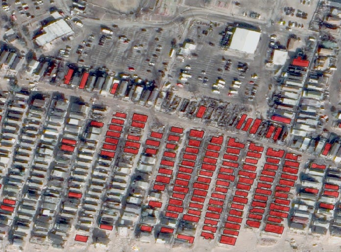
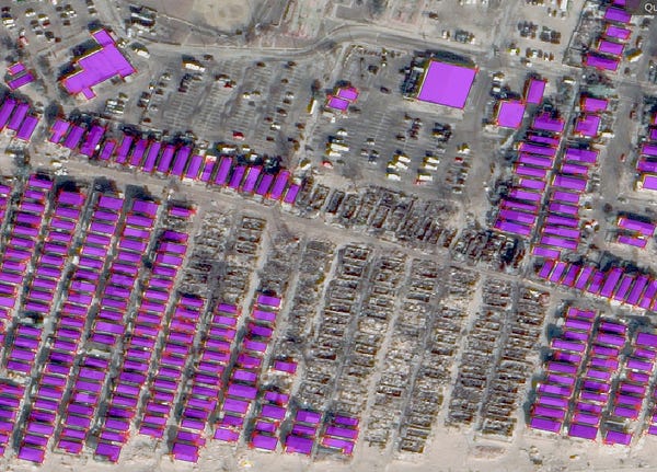
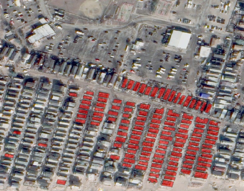
As a result, we can see a very impressive new mask that describes houses that have survived the hurricane (Figure 15) and a vector of the ruined buildings (Figure 16).
Clik here to view.

Clik here to view.
Clik here to view.
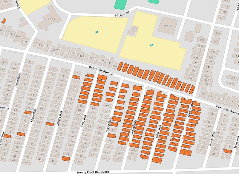
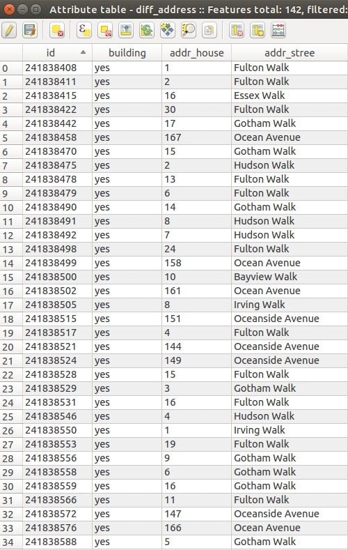
After we have found the ruined houses, we can also pinpoint their location. For this task OpenStreetMap comes in handy. We have installed an OSM plugin in QGis and added an OSM layer to the canvas (Figure 17). Then, we added a layer with the destroyed houses and we can see all their addresses. If we want to get a file with the full addresses of the destroyed buildings we have to:
- In QGis use Vector / OpenStreetMap / Download the data and select the images with the desired information.
- Then in QGis use Vector / OpenStreetMap / Import a topology from XML and generate a DataBase from the area of interest.
- QGis / Vector / Export the topology to Spatialite and select all the required attributes. (Figure 18)
Clik here to view.
Clik here to view.
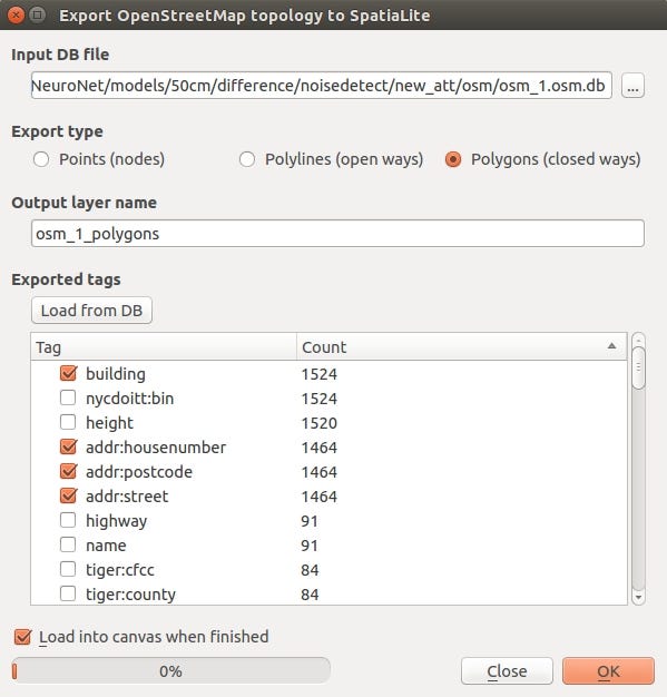
As a result, we can get a full list, with addresses, of the destroyed buildings (Figure 19).
Clik here to view.
If we compare these two different approaches to building recognition, we notice that the CNN-based method has 78% accuracy in detecting destroyed houses, whereas the Laplace filter reaches 96.3% accuracy in recognizing destroyed buildings. As for the recognition of existing buildings, the CNN approach has a 93% accuracy, but the second method has a 97.9 % detection accuracy. So, we can conclude that the flat surface recognition approach is more efficient than the CNN-based method.
The demonstrated method can immediately be very useful and let people compute the extent of damage in a disaster area, including the number of houses destroyed and their locations. This would significantly help while estimating the extent of the damage and provide more precise measurements than currently exist.
For more information about EOS Data Analytics follow us on social networks: Facebook, Twitter, Instagram, Linkedin.
图像处理一定要用卷积神经网络?这里有一个另辟蹊径的方法
| 本文作者:恒亮 | 2017-01-09 20:44 |
近年来,卷积神经网络(CNN)以其局部权值共享的特殊结构在语音识别和图像处理等方面得到了快速发展,特别是大型图像处理方面,更是表现出色,逐渐成为了行业内一个重要的技术选择。
不过,好用并不代表万能。这里雷锋网从一个卫星图像分析的具体实例出发,介绍了CNN建模和本地拉普拉斯滤波这两种分析技术的效果对比,最终我们发现,本地拉普拉斯滤波的效果反而更好。
卷积神经网络
为了从卫星图像中分析和评估一项自然灾害造成的损失,首先需要得到相关地理区域实时的高分辨率的卫星图像,这是进行后续所有分析的数据基础。目前,除了Google Earth之外,最方便也最经济的数据来源就是OSM(OpenStreetMap)开源地图计划。该计划于2004年在美国创立,类似于维基百科,鼓励全球用户自由无障碍地分享和使用地理位置数据。
由于OSM提供的是矢量数据(Vector Data),为了便于空间分析和地表模拟,因此需要利用GDAL(Geospatial Data Abstraction Library)库中的 gdal_rasterize 工具将其转化为栅格数据(Raster Data)。
雷锋网(公众号:雷锋网)注:矢量数据和栅格数据都是地理信息系统(GIS)中常见的分析模型。其中栅格结构是以规则的阵列来表示空间地物或现象分布的数据组织,组织中的每个数据表示地物或现象的非几何属性特征。特点是属性表现明显,便于空间分析和地表模拟,但定位信息隐含。而矢量数据结构是通过记录坐标的方式尽可能精确地表示点、线和多边形等地理实体,坐标空间设为连续,允许任意位置、长度和面积的精确定义。特点是定位信息明确,但属性信息隐含。
得到栅格数据之后,下一步是利用Caffe开源框架和CNN模型对系统进行训练。如图所示为CNN模型的一种参数设置。
Image may be NSFW.
Clik here to view.
CNN模型的一种参数设置
利用大量数据训练得到的卷积神经网络模型处理灾后的图像,识别出的受灾房屋情况如图所示(图中白色色块代表房屋,具体可对比后面拉普拉斯滤波的处理结果)。
Image may be NSFW.
Clik here to view.
Image may be NSFW.
Clik here to view.
CNN的分析结果,左图为灾前的图像,右图为灾后的图像
拉普拉斯滤波
另一种方式是跨过GDAL转换,利用拉布拉斯滤波直接在矢量数据的基础上进行分析。
具体方法是:对比灾前和灾后两张图像,识别房屋的变化和两个图像的重叠部分,从而对受灾程度做出评估。本例中将对比阈值设为10%,即如果灾后图像中某个房屋的面积小于灾前面积的10%,那么就判定这一房屋已经被损毁。
需要注意的是,这里用到了两个重要的滤波器。一个是拉普拉斯滤波,作用是识别出图像中所有突出的不平整的部分(这里即所有的房屋轮廓),然后将其标记并绘制出来。另一个是设置为10%的“噪声”滤波,即对比灾前和灾后的图像,按照10%的阈值过滤出受灾的房屋。
相比CNN的方法,这里用到了该问题的一个独特属性,即房屋总是高于地面的,而且利用多边形方块可以清晰地标出其轮廓。
Image may be NSFW.
Clik here to view.
拉普拉斯滤波模型
如图所示为 Matlab 建模的本地拉普拉斯滤波窗口,其中“img”变量为包含4个通道的原始图像,其中除了RGB三原色通道外,还有一个额外的 Alpha 通道,用来标明每个像素点的灰度信息。而变量“img1”是与“img”完全相同的图像,只是被滤除了 Alpha 通道。
Image may be NSFW.
Clik here to view.
拉普拉斯滤波结果,红色色块为房屋
Image may be NSFW.
Clik here to view.
OpenCV滤波模型
如图所示是利用OpenCV开源计算机视觉库实现的第二个滤波器,以及滤波结果,可以看到受灾房屋被清晰地滤出了(相对CNN来说)。
Image may be NSFW.
Clik here to view.
OpenCV滤波结果
如图所示为两个滤波器的作用效果。
Image may be NSFW.
Clik here to view.
两个滤波器的综合作用结果
在输出结论前,还需要将此时的滤波结果与灾前图像进行最后的对比,用14%的面积阈值判定最终的受灾房屋情况,以避免此前计算中引入的误差。
Image may be NSFW.
Clik here to view.
14%面积的阈值判定
如图所示,其中黄色为拉普拉斯滤波的结果,绿色为灾前图像。
识别出受损房屋之后,借助灾前OSM数据库的帮助,还可以通过QGIS工具方便地导出每间受损房屋的地址列表信息。具体步骤是:首先将灾前OSM数据导入QGIS平台最为底层信息,然后导入之前的分析结果,通过对比得到受损房屋的具体位置,然后导入一份XML格式的拓扑结构说明文件,接着利用SpatiaLite数据库管理平台就能根据需要导出一份具体房屋和地址相对应的列表信息。
Image may be NSFW.
Clik here to view.
利用 QGIS 和 SpatiaLite 导出地址列表
最终对比发现,以CNN技术为核心的受灾房屋识别准确率只有78%,而拉布拉斯滤波则高达96.3%。另外,拉布拉斯滤波的这一优势在灾前建筑的识别上也得到了延续,其正常建筑的识别准确率高达97.9%,而相比之下CNN只有93%。到这里结论已经很明显了:基于平整度识别的拉普拉斯滤波最终效果要优于基于大数据训练的CNN卷积神经网络。
需要指出的是,上文提到的拉普拉斯滤波法的重要意义并不局限于其技术实现本身,这种根据特殊问题采取特殊处理方法的应对策略,也同样值得我们思考。
来源:medium,由雷锋网编译
Image may be NSFW.
Clik here to view.
Clik here to view.