Object Detection in Satellite Imagery, a Low Overhead Approach, Part I
The promise of detecting and enumerating objects of interest over large areas is one of the primary drivers of interest in satellite imagery analytics. Detecting small objects in cluttered environments over broad swaths is a time consuming task for analysts, particularly given the ongoing growth of imagery data. A number of integrated pipelines using convolutional neural nets (FasterRCNN, YOLO) have proven very successful for detecting objects such as people, cars or bicycles in cell phone pictures. These methods are not optimized to detect small objects in large images, and often perform poorly when applied to such problems. Adapting these methods to the different scales and objects of interest in satellite imagery shows great promise, but is a research area still in relative infancy and one to be explored later. In this paper we discuss a simpler approach using pre-filters and sliding windows paired with histogram of oriented gradient (HOG) based classifiers.
While the sliding window approach may be considered a brute force approach, it is also simple to implement and effective in certain problems. Furthermore, all of the work shown here is run on a laptop using open source software [1, 2, 3]; no GPU, high performance computing cluster, or proprietary software licenses required. We apply the sliding window approach to a maritime domain awareness problem and attempt to enumerate ships at anchor as well as in harbor. In later posts we will detail an increasingly sophisticated classification approach and compare it with sliding windows paired with neural network classifiers.
1. Sample Scene
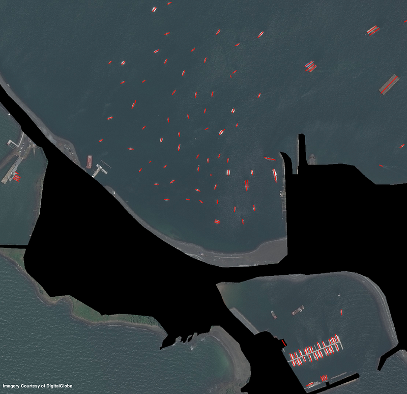
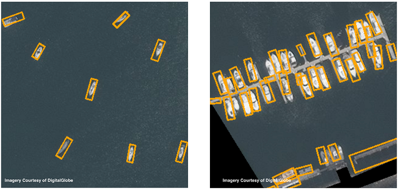
For demonstration purposes, we choose a 2200 x 2200 pixel subset of the DigitalGlobe (DG) WorldView2 0.5m ground sample distance (GSD) validation image taken near the Panama Canal (see the datasets post, Section 4 for more information). Raw DigitalGlobe cutouts are roughly 50 times larger than this cutout, at ~16,000 x 16,000 pixels. The diverse maritime scene selected contains terrestrial regions, boats in open water, and moored boats. There are 112 boats total, 1/3 of which are in harbor, a handful are anchored together, and the remainder are in open water (Figure 1).
2. Preprocessing
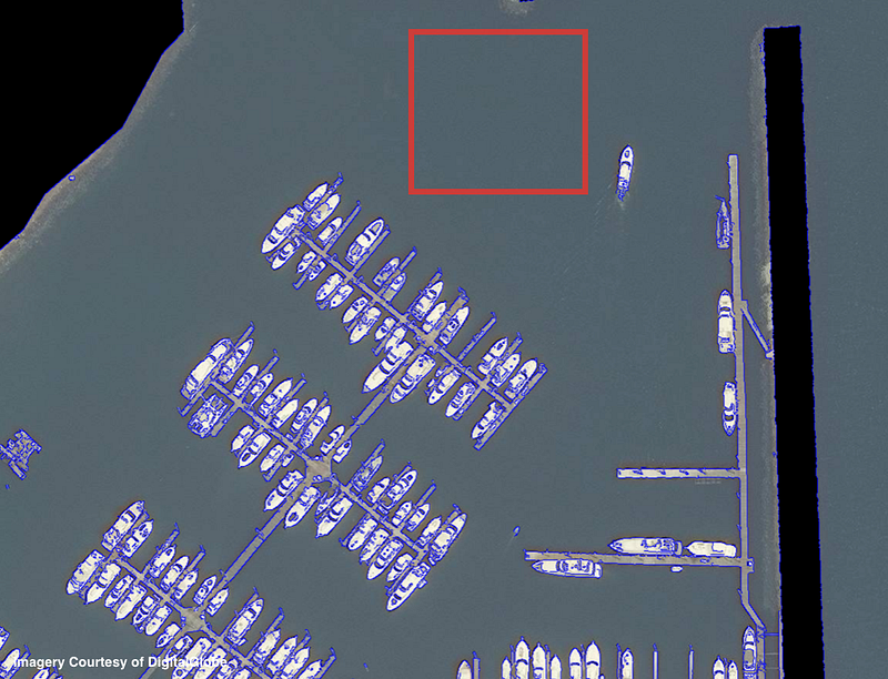
When searching for detailed objects the human eye tends to skim over featureless regions and hone in on more complex scenes. Efficient preprocessing techniques should strive to emulate this process by discarding regions with an obvious lack of notable features and flag complex regions for further analysis. Myriad methods exist for such processes: image segmentation, thresholding, masks, corner detection, SURF, gradients, contours, Canny edge detection, etc. We focus on image masks and Canny edge detection as powerful techniques for maritime scenes. Shape files fromOpenStreetMap can be used to construct a terrestrial mask, leaving only maritime regions. Open water is relatively featureless when viewed from above, and so Canny edge detection can be used to identify areas of interest (Figure 2). Edge detection can be very useful in sparse scenes, though image noise such as whitecaps or haze (which reduces image contrast) can severely limit the utility of using Canny edges as a pre-filter.
3. Classifier Training Data and Hard Negative Mining
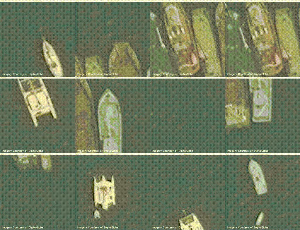
For boat detection heading classification purposes we use the dataset defined in our datasets post and follow the same approach to building a classifier as that described in the boat heading post. Those posts sought to differentiate boats from background images, and determine the heading of positive results. Our current goal of object localization is slightly different in that we want to draw a bounding box around the entirety of each positive detection. Initial runs of the classifier pipeline defined in the boat heading post yield many partial boats or dock regions classified as positive results. We deem these false positives, feed them back into the classifier defined below, and retrain. This process is called hard negative mining and has the potential to greatly reduce false positives, particularly when applied multiple times. We only run a single iteration of hard negative mining as proof of concept, but in a deployed environment one would likely continually feed in false positives to the system to successively refine the classifier.

4. Multiple Binary Classifiers
The HOG+PCA+LogReg classifier defined in the boat heading post works well for boat heading classification, yet in initial experiments it struggles to accurately locate boats. The 73-class classifier cannot adequately disentangle docks and partial boats from full boats. To address this issue we train a corpus of 72 binary boat/no-boat random forest (RF) classifiers, one for each 5-degree rotation. Classification accuracy on boat headings (using the exact same training and testing data as the boat heading post) is nearly identical to the HOG+PCA+LogReg classifier, though differentiation between partial boats and full boats is significantly improved. Training the RF classifier set takes 145 seconds on a single CPU (no GPU needed).
Run time is of great importance for object detection over large regions. Extracting the HOG descriptor takes 0.49 milliseconds per window; fitting the multi-class logistic regression classifier takes a mere 0.008 milliseconds per image, while applying the 72 binary random forest classifiers adds 0.33 milliseconds per image. The multi-class classifier obviously is far faster than the 72 binary classifiers, though HOG feature extraction is still the slowest step. These evaluation times are for CPU computation, and should enjoy marked speed improvements if optimized for GPU computation. All told, the HOG+RF classifier takes ~0.8 milliseconds per image to evaluate. For comparison, on the CosmiQ GPU server (CosmiQ is running an NVIDIA DIGITS DevBox with four TitanX GPUs), each evaluation of an AlexNet-based neural network model takes 10 milliseconds.
5. Sliding Window Introduction
Sliding window approaches are simple in concept, a bounding box of the desired size(s) slides across the test image and at each location applies an image classifier to the current window (see Figures 4, 5).

6. Window Cutouts
Satellite imagery is unique from most other imagery types in that pixels remain a static physical size, known as ground sample distance (GSD). For example, if one is searching for a 45m ship in DigitalGlobe data at 0.3m GSD, one need only look for objects of length ~150 pixels. The sliding window box sizes are therefore determined by the scales of objects of interest. Given the diversity of ship lengths in our test image, we select window sizes of [140, 100, 83, 66, 38, 22, 14, 10] meters.
The total number of sliding windows is a function of the number of scales searched, with smaller scales imparting a much larger computational toll given the larger number of windows. Searching for small objects is computationally expensive, as the number of windows is a quadratic function of window size (one can extract approximately four times as many 10×10 windows as 20×20 windows from a given image).
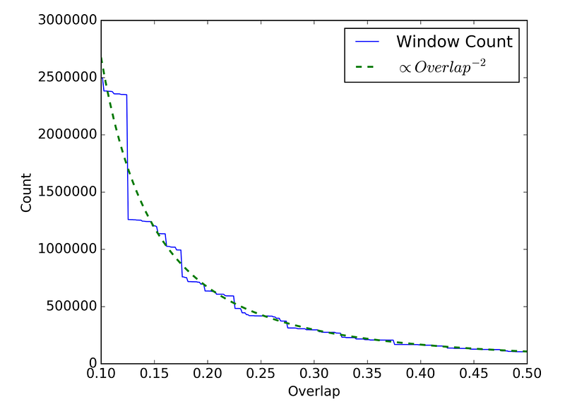
The total number of windows also depends heavily on the level of overlap between windows. Effective localization for closely spaced objects requires a high degree of overlap between sliding windows. We find that a step of 1/6 of the bin size works well. The total number of windows to analyze is strongly dependent on the overlap fraction (proportional to the square inverse of the overlap fraction).
The simple Canny edge detection preprocessing discussed in Section 2 significantly reduces computational requirements. Iterating through the test image and keeping only those images flagged by the edge detection algorithm yields 26,000 bins (a 30x reduction) after a run time of 3.8 seconds on a single CPU. Computing the HOG feature descriptors takes another 12.8 seconds, and classification takes 9.6 seconds, for a total of ~26 seconds for the DG sub-image. This translates to ~15 minutes for each full DigitalGlobe image on a single CPU.

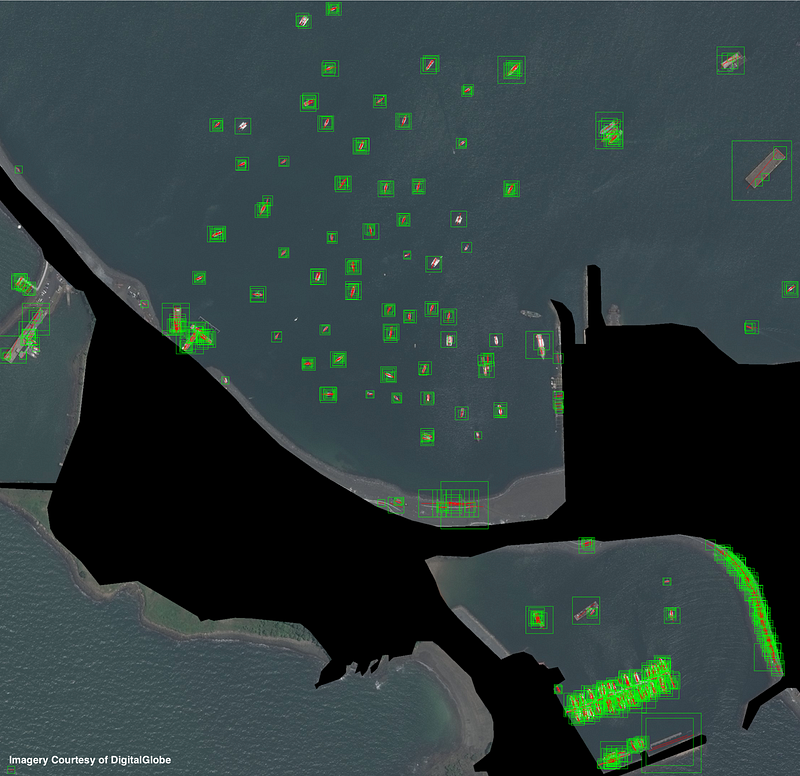
7. Sliding Window Results
8. Square Non-Max Suppression
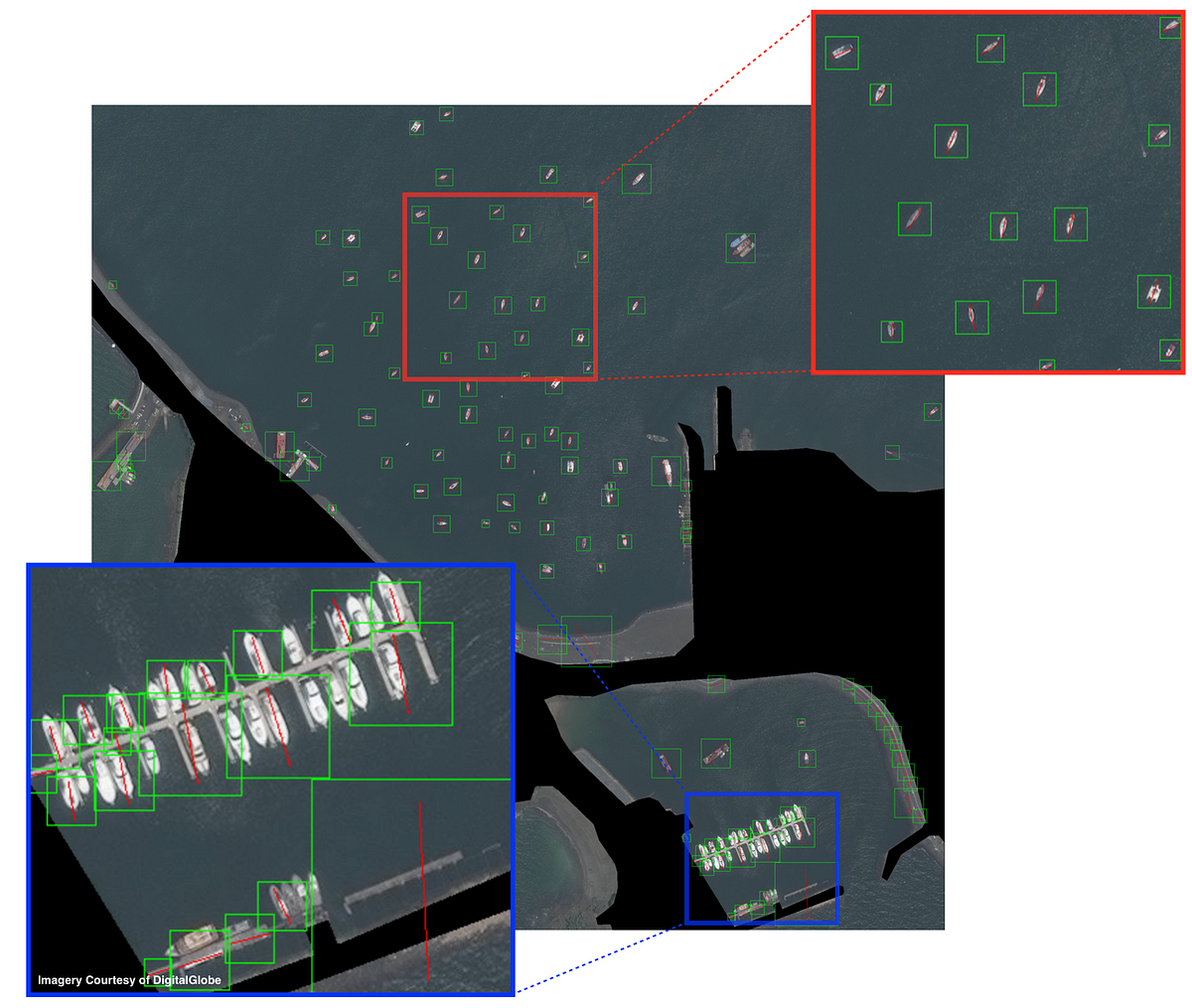
Non-maximum suppression is a method for collapsing overlapping detections into a single detection (see here for an excellent example). The method works by discarding detections with an overlap greater than a specified threshold with previously seen detections. Traditionally, non-max suppression is applied to rectangular bounding boxes oriented in cardinal directions. This method is very fast, and takes a mere 16 milliseconds for our 951 detections.
9. Conclusions
In this post we showed how to combine Canny edge detector pre-filters with HOG feature descriptors, random forest classifiers, and sliding windows to perform object detection on satellite imagery. Our only computing resources are a laptop and open source software packages.
Searching for boats of length [140, 100, 83, 66, 38, 22, 14, 10] meters, the entire classification pipeline takes < 30 seconds for our test image, translating to ~15 minutes for a full 8×8 kilometer DigitalGlobe image on a single CPU. This run-time could be greatly reduced by looking only for longer ships. For example, only searching for boats of length greater than 20m takes only ~three minutes for a full DigitalGlobe image, a marked decrease from 15 minutes.
Harbor regions are a challenge for the Square Sliding Window + HOG + RF approach, yet open-water accuracy is quite high when non-max suppression is used to combine overlapping detections. In Part II of this series, we will discuss improved methods for collapsing overlapping detections, and quantify performance.
Object Detection in Satellite Imagery, a Low Overhead Approach, Part II
In this post we show improved results for object detection in congested regions via a novel method for collapsing overlapping detections using heading information. We also demonstrate that for satellite imagery object detection, rotated bounding boxes have advantages over rectangles oriented in the cardinal directions.
The promise of detecting and enumerating objects of interest over large areas is one of the primary drivers of interest in satellite imagery analytics. Detecting small objects in cluttered environments over broad swaths is a time consuming task, particularly given the ongoing growth of imagery data. In theprevious post, we showed how to perform object detection on satellite imagery with just a laptop and open source software by combining Canny edge detector pre-filters with HOG feature descriptors, random forest classifiers, and sliding windows. We found that performance in open-water localization is quite good when square non-max suppression is used to combine overlapping detections, though congested regions remain a challenge.
1. Object Detection Pipeline
Recall from Part I that our object detection pipeline combines Canny edge detector pre-filters with HOG feature descriptors, random forest classifiers, and sliding windows. This process takes < 30 seconds for the image shown in Figure 1.

Square non-max suppression collapses some overlapping detections in open water, but works poorly in congested regions (see Figure 2).

2. Performance Evaluation
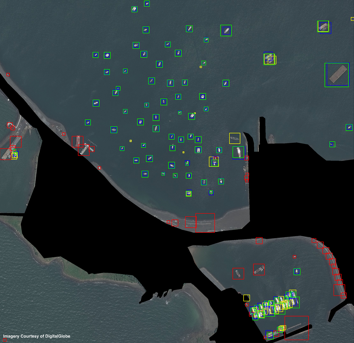
We can combine the output of non-max suppression shown in Figure 2 with the ground truth labels of Figure 1 in Part I to evaluate the performance of our object detection methodology. We compute and plot three categories: false positives, false negatives, and true positives. We define a true positive as having a Jaccard index (also known as intersection over union) of greater than 0.25. A Jaccard index of 0.5 is often used as the threshold for a correct detection, though as in Equation 5 of ImageNet we select a lower threshold since we are dealing with very small objects.
3. Congested Region Overlap Suppression
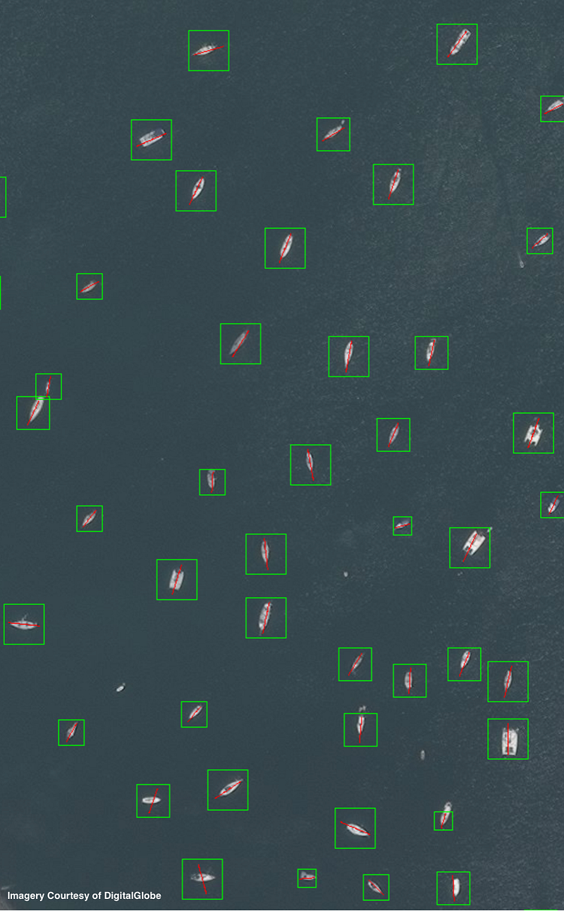
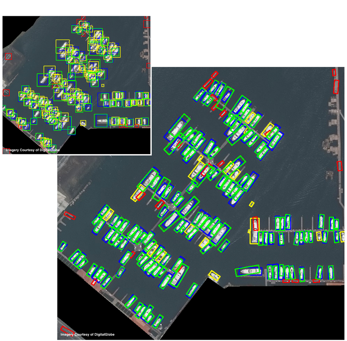
Figure 3 illustrates the poor performance in congested regions of standard rectangular bounding boxes oriented in cardinal directions. In order to improve results, we take advantage of the heading information provided by our classifier and knowledge of object aspect ratio to create an improved method for overlap suppression using rotated rectangular bounding boxes. This method greatly improves localization in crowded regions. Computing rotated rectangular overlap suppression for the 951 detections takes 3.3 seconds.
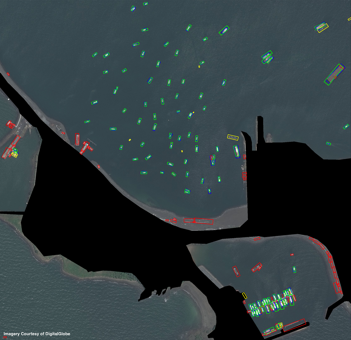
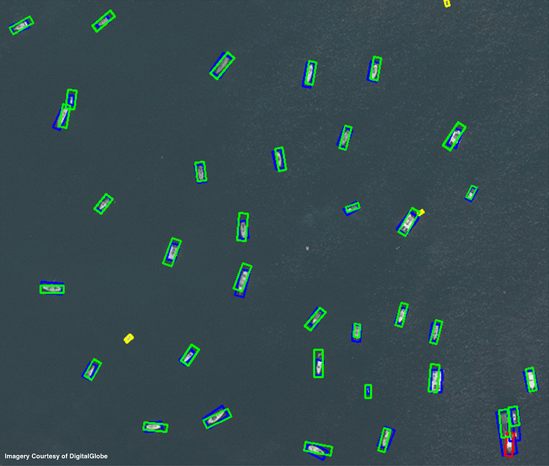
As a check of our results in Figure 5, we apply the object detection pipeline to three more areas of interest with hand-labelled ground truth. Results are varied, and described in figure captions.


9. Conclusions
In this post we showed results of combining Canny edge detector pre-filters with HOG feature descriptors, random forest classifiers, and sliding windows to perform object detection on satellite imagery using only a laptop and open source software packages. We utilize the heading information provided by our classifier to introduce a new technique for rotated rectangular overlap suppression that greatly improves results in crowded regions.
Searching for boats of length [140, 100, 83, 66, 38, 22, 14, 10] meters, the entire classification pipeline takes < 30 seconds for our test image, translating to ~15 minutes for a full 8×8 kilometer DigitalGlobe image on a single CPU. This run-time could be greatly reduced by looking only for larger boats. For example, searching for boats of length greater than 20m takes only ~3 minutes for a full DigitalGlobe image, a marked decrease from 15 minutes.
The detection pipeline performs very well in open water on boats of similar size to the training set median size (AOI2: precision=0.97, recall > 0.92). Open water detection is less impressive for larger boats in choppy seas due to the lower contrast between object and background and fewer training images at this scale (AOI3: precision=0.70, recall=0.54); one could improve performance by relaxing detection thresholds and only looking for boats greater than 50m in length. Performance in harbor is quite high (AOI4: precision=0.84, recall=0.87), with the number of proposed items within 5% of ground truth.
For low background images the HOG + sliding window approach appears a very compelling option, particularly given its speed and ability to elucidate dense regions with closely spaced objects. Forthcoming posts will explore neural network based approaches to object detection in satellite imagery. Though neural networks and deep learning have enjoyed great success as of late, few neural network models are optimized to localize small, densely packed objects in large images. It will be interesting to see how advanced deep learning techniques compare to the low computational overhead approach proposed here.